The model we’ve built so far represents an ideal operating scenario. Material flows smoothly, equipment runs continuously, and production occurs at the maximum possible rate. While this is useful for understanding the structure of the system, real operations rarely behave this way.
To make the model reflect real-world performance, we need a way to represent events that interrupt production. In ReliaSim, this is done using interrupts. Interrupts introduce downtime and variability so the model can simulate how failures, maintenance, or other disruptions affect flow.
Each interrupt is defined by two distributions: Time to Failure and Time to Repair. The Time to Failure distribution describes how long the process operates before a specific failure occurs. It represents the statistical “survival time” of that condition. The Time to Repair distribution defines how long the process remains down before it can return to operation.
Time to Failure behavior generally falls into two categories: competing and cumulative.
With competing failures, the failure timer resets whenever any interrupt occurs. This reflects situations where maintenance or repair actions address multiple potential issues at once, even if only one actually caused the stop. A common example is a machine with several wear components that are all replaced when any one of them fails.
With cumulative failures, the timer does not reset when other interrupts occur. Instead, the remaining time continues from where it left off. This models wear mechanisms that are only corrected when that specific component fails, such as a part that gradually degrades and is not replaced during unrelated maintenance.
Time to Repair distributions are tied directly to the failure being addressed. Each failure mode can have its own repair behavior, allowing the model to reflect differences between quick resets, longer maintenance tasks, or complex recovery efforts.
By introducing interrupts, the model moves beyond ideal capacity and begins to represent how reliability, maintenance, and variability shape actual production performance.
For more complex, and real world models, interrupts are going to be based on the history of the process in question. ReliaSim has fitting tools to help take existing data and get a good representation for simulation, but the use and functions of this tool are outside the scope of this model. For the time being, let's introduce some fairly straightforward interrupts using largely default settings.
For our first node, the filler, let's assume we have two interrupts. One could be a nozzle clog and the other could be a jar jam. If we were to treat this as a maintenance plan where the nozzles are cleaned and the jars are checked or staged whenever either event occurs, these would be competing interrupts. ReliaSim defaults to a Weibull distribution for both the time to failure and the time to repair when a new interrupt is added. This is pretty reasonable for our purposes, so let's leave it as is. For illustrative purposes, let's assume that the jar jam has a longer time to repair than the nozzle clog. Let's double the first parameter, λ, of this distribution. If you select the converter editor on the right hand side, hit edit on the jar filler, and then add interrupts and fill in the data as described, you should end up with this.
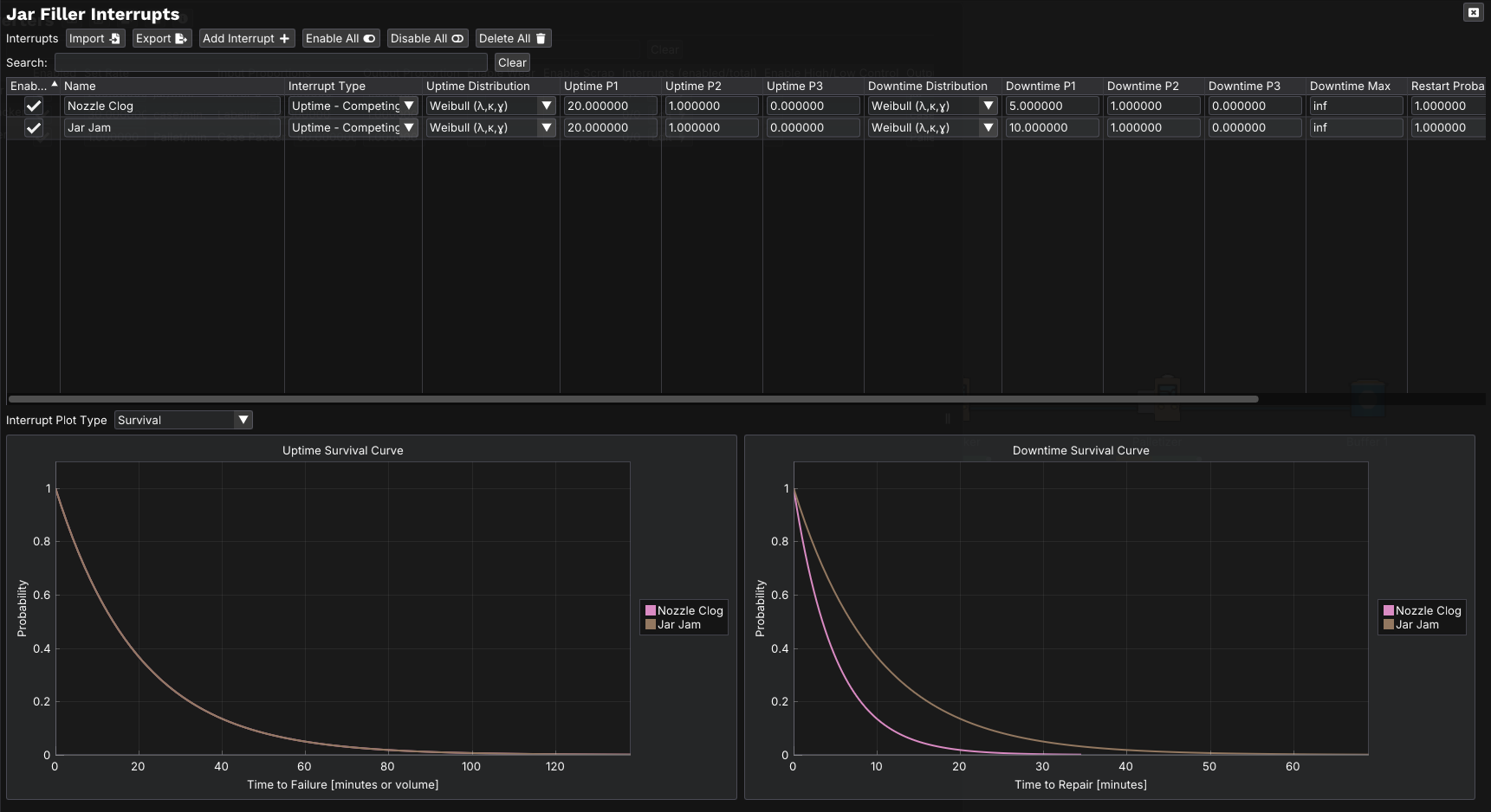
You can also import or export interrupt data as *.csv files.
for the sake of our example, let's also add a default interrupt to the capper and case packer. Our model now looks like this.
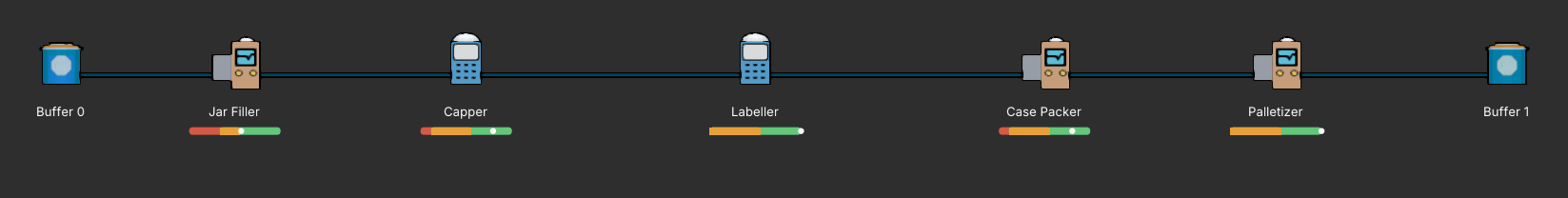
we can also see that our efficiency has dropped to around 44%, This shows the real impact of our interrupts. the gauges under each node illustrate the efficiency of that node on it's own. In the next section, we'll conduct some experiments to better understand the model we're simulating.